GAN for Speech Enhancement

[TOC]

SEGAN: Speech Enhancement Generative Adversarial Network

INTERSPEECH 2017

Universitat Politecnica de Catalunya, Barcelona, Spain (西班牙，巴塞罗那，加泰罗尼亚理工大学)

G的结构

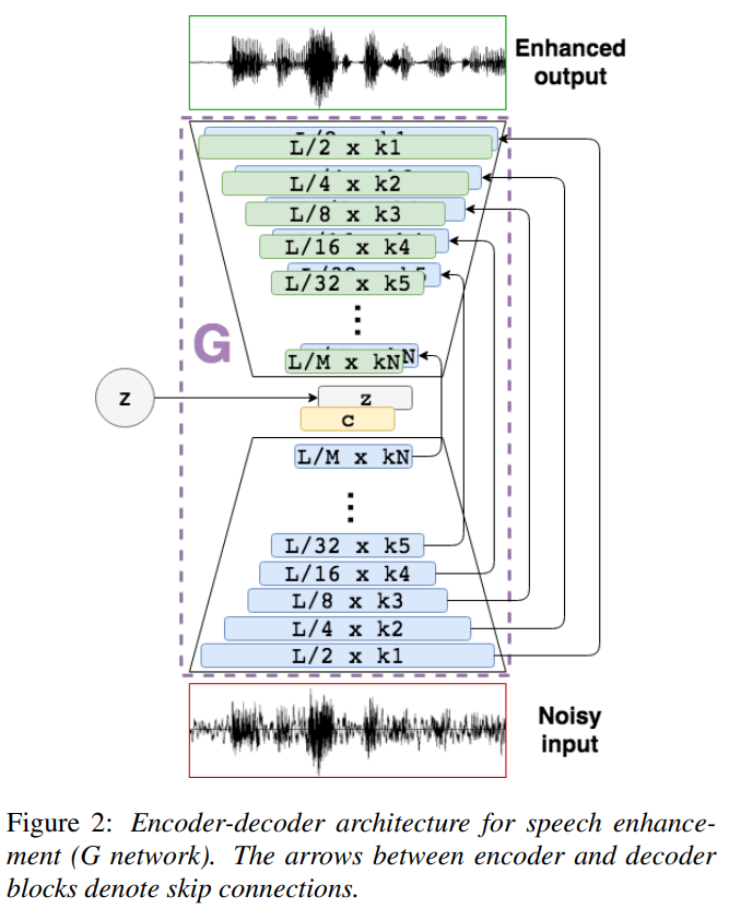
含有SkipConnection和encoder-decoder的U-Net结构，encoder与decoder均采用一维全卷积，无BN

G的输入输出

16kHz、16384点时域波形输入encoder得到latent vector c，c与正态随机噪声concat进入decoder，最后输出enhanced时域波形

G的loss

D的结构

类似G的encoder，有BN

D的输入输出

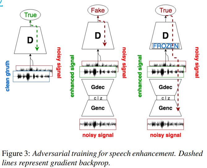
将enhanced wave和noisy wave concat或将clean wave和noisy wave concat输入D，得到一个概率值

D的loss

数据集及数据预处理

Voice Bank+DEMAND数据集

16kHz采样率、以16384点为一帧，帧与帧之间有0.5的overlap，逐帧进行增强

文章的创新点

GAN for SE的开山之作？

项目地址

https://github.com/santi-pdp/segan

Conditional Generative Adversarial Networks for Speech Enhancement and Noise-Robust Speaker Verification

INTERSPEECH 2017

Aalborg University (奥尔堡大学)

G的结构

含有SkipConnection和encoder-decoder的U-Net结构，encoder与decoder均采用二维全卷积，无正态随机噪声

G的输入输出

输入[256,256,1]的stft幅度谱，输出[256,256,1]的增强谱

G的loss

vGAN的G_loss加上l1_loss

D的结构

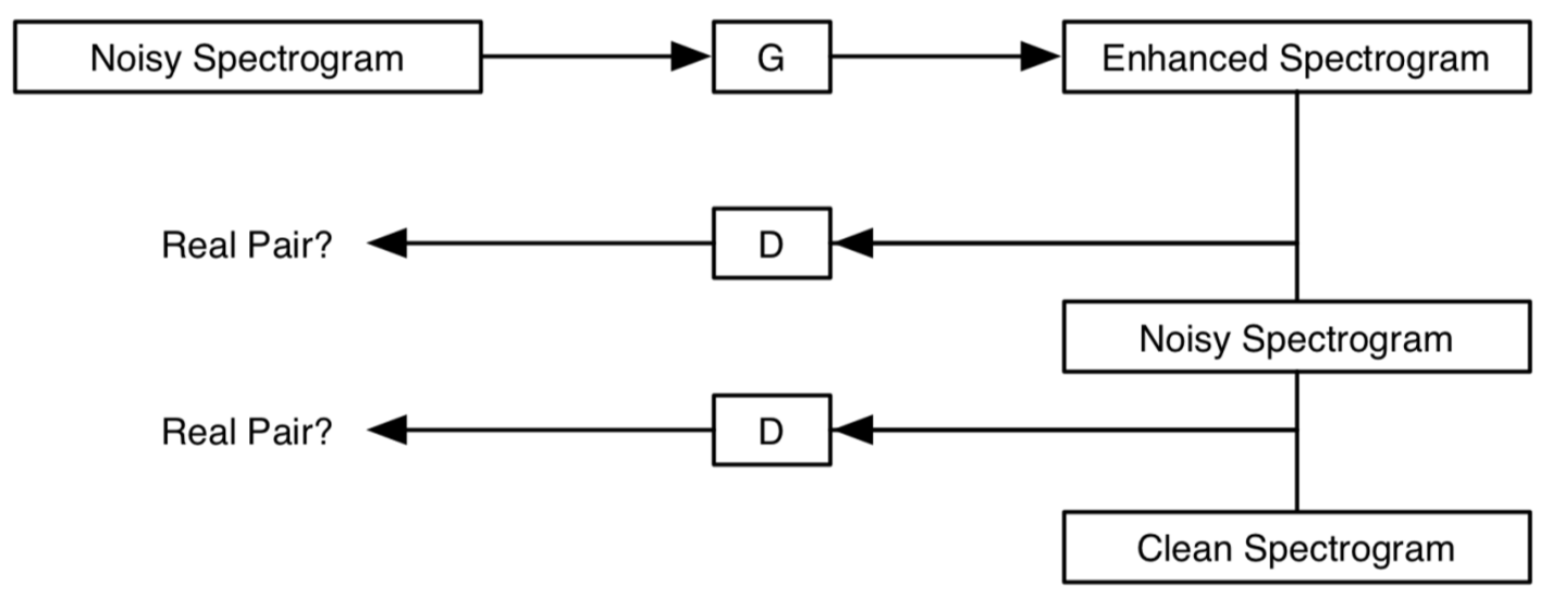
类似G中encoder，使用PatchGAN思想

D的输入输出

将enhanced stft幅度谱和noisy幅度谱concat或将clean幅度谱和noisy幅度谱输入D，得到一个概率值

D的loss

cGAN的D_loss

数据集及数据预处理

TIMIT和RSR2015及一些噪声数据集

16kHz采样、一帧32ms、overlap 16ms的stft，得到[256,257]的stft谱，去掉最高的频率段，得到[256,256,1]的幅度谱

文章的创新点

cGAN思想

这篇文章的实现主要基于Image-to-Image Translation Using Conditional Adversarial Networks和Unsupervised representation learning with deep convolutional generative adversarial networks

Generative Adversarial Network-based Postfilter for STFT Spectrograms

INTERSPEECH 2017

NTT Communication Science Laboratories (日本电报电话公司通信科学实验室)

G的结构、输入输出与D的结构、输入输出

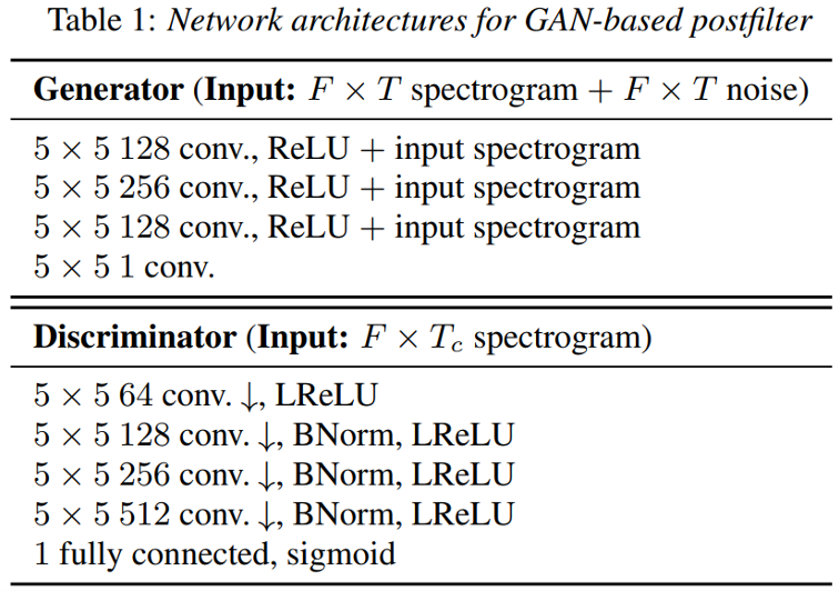
Made three changes to the regular GAN architectures by using conditional, residual, and convolutional networks for postfiltering:

Conditional: cGAN with stochastic noise
Residual: $G(x,y)=y+R(x,y)$, where $R$ represents residual texture
Convolutional: design the G as a fully convolutional network (FCN) that allows input segments to take an arbitrary length

损失函数

数据集及数据预处理

Blizzard Challenge 2011

Normalized spectrograms to zero-mean and unit-variance for each dimension
Divided the spectrogram into four frequency bands (1,320) (257,576) (513,832) (769,1024)
After enhanced, connected the bands with the hamming-window function where the window width was 128

文章的创新点

Partition: We first divide the spectrogram into $N$ frequency bands, each of which ranges from the $f^s_i$-th to $f^e_i$-th frequency, where $N$ is the number of bands and $i = {1, . . . , N}$. The overlap between the $i$-th and $i + 1$-th bands is set at $v_i$, i.e., $vi = f^e_i − f^s_{i+1}$. We use the overlap representation to smoothly concatenate the individual bands afterwards.
Postfiltering: We reconstruct the individual bands using the GAN-based postfilter trained for each band. The spectrogram in each band is not only lower dimensional but also has a more homogeneous structure than the entire spectrogram; therefore, we expect that it is easier to model.
Concatenation: To smoothly connect the reconstructed spectrograms, we apply a window function (e.g., hanning, hamming, or Blackman) to both ends of each band before connection, where the window width is $2v_i$ and half of the window function is applied to each end. This method works well. In preliminary experiments, we also tested a model in which the spectrograms are divided and connected without overlap. In this model, the reconstructed spectrogram tends to have discontinuity between the bands, causing a popping sound.

由于这篇文章的目的是对TTS合成谱做增强，所以文中还提出了一个prior acoustic model，这里不详说

Time-Frequency Masking-Based Speech Enhancement Using Generative Adversarial Network

ICASSP 2018

Dhirubhai Ambani Institute of Information and Communication Technology, Gandhinagar, India (印度甘地纳加尔信通研究所德鲁拜-安巴尼学院)

G的结构

G consists of three hidden layers. Each layer had 512 units with Rectified Linear Unit (ReLU) activation. The output layer had 64 units to predict T-F mask implicitly. Sigmoid activation was used to limit the output mask values between 0 to 1.

D的结构

The D network had three hidden layers with 512 units in each layer. However, the units has tanh activation function. The output layer had single unit with sigmoid activation.

损失函数及输入输出

# construct the model
esti_spec = generator(x, weights, biases) # x is the noisy log gammatone spectra
D_real, D_logit_real = discriminator((y_-MEAN)/STD) # y_ is the clean log gammatone spectra
D_fake, D_logit_fake = discriminator((esti_spec-MEAN)/STD) # MEAN and STD is the mean and std of y_

# calculate the loss
D_loss_real = tf.nn.sigmoid_cross_entropy_with_logits(labels=tf.ones_like(D_logit_real), logits=D_logit_real)
D_loss_fake = tf.nn.sigmoid_cross_entropy_with_logits(labels=tf.zeros_like(D_logit_fake), logits=D_logit_fake)

D_loss = tf.reduce_mean(D_loss_real) + tf.reduce_mean(D_loss_fake)
G_RMSE = 0.5*(tf.reduce_mean(tf.square(tf.subtract(y_, esti_spec))))
G_gan = tf.reduce_mean(tf.nn.sigmoid_cross_entropy_with_logits(labels=tf.ones_like(D_logit_fake), logits=D_logit_fake))
G_loss = G_gan + G_RMSE

数据集及数据预处理

Voice Bank + DEMAND

文章的创新点

无，我觉ICASSP的文章普遍没有INTERSPEECH的好，这篇文章github上有repo，但缺少一些函数所以用不了

项目地址

https://github.com/Neil-Shah/GANs-for-Speech-Enhancement

Exploring Speech Enhancement With Generative Adversarial Networks For Robust Speech Recognition

ICASSP 2018

UC San Diego Department of Music (加州大学圣地亚哥分校音乐系) and Google

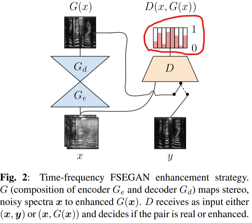
G的结构

含有SkipConnection和encoder-decoder的U-Net结构，encoder与decoder均采用二维全卷积，无BN，无正态随机噪声

G的输入输出

128x128的time-frequency spectra

D的结构

类似encoder

D的输入输出

基于cGAN的思想输入pair，对每一个timestep输出一个概率

损失函数

PS: 去掉随机正态噪声z

数据集及数据预处理

Wall Street Journal (WSJ) corpus

SI-284 set and eval92 set

128ms windows with 50% overlap stft得到[128,128]的time-frequency spectra

文章的创新点

研究了将GAN for SE应用于ASR model的效果
实验表明，对于ASR较简单的回归方法可能优于基于GAN的增强 (hhhh，服了)
D的基于timestep的输出挺有意思

这篇文章的实现主要基于Image-to-Image Translation Using Conditional Adversarial Networks

记录一下这篇文章中给出的log Mel filterbank spectra的计算：

magnitude stft spectrum with window size of 32ms and hop size of 10ms
triangular windows for a bank of 128 filters, where filter center frequencies are equally spaced on the Mel scale between 125 Hz and 7500 Hz
logarithm of the output and normalize each frequency bin to have zero mean and unit variance (我觉得是否使用normalization视情况而定)

On Adversarial Training And Loss Functions For Speech Enhancement

INTERSPEECH 2018

Ohio State University (俄亥俄州立大学)

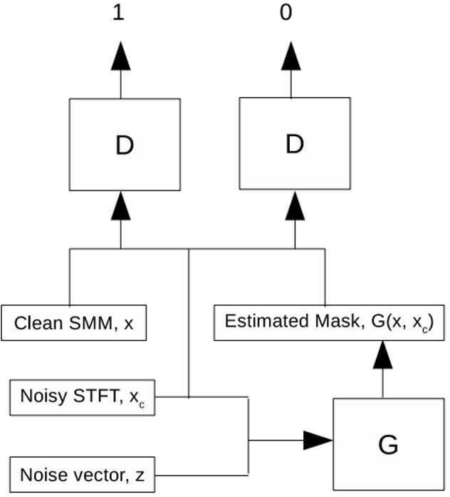
G的结构与D的结构

Fully connected DNN

All DNNs use 3 hidden layers. Batch normalization is used before every layer except the output layer of the discriminator and the input layer of the generator. A dropout rate of 0.2 is used for all the hidden layers. The discriminator uses leaky ReLUs at the hidden layers and no activation at the output layer. The generator uses parametric ReLUs at the hidden layers and the output layer activation is determined by targets.

G的输入输出

Input: concatenation of two vectors, $x_c$ and $z$, where $x_c$ is the STFT magnitude of noisy speech and $z$ is a randomly sampled noise vector from a normal distribution

Output: $G(z, x_c)$ is the estimated SMM

D的输入输出

输入Mask pair，输出概率

损失函数

在cGAN的基础上探索l1_loss和l2_loss

数据集及数据预处理

文章的创新点

For comparison between L1 loss training and adversarial training, tanh is used at the output layer of the generator. For L1 and L2 loss comparison, ReLU is used for STFT magnitude and SMM, and sigmoid is used for IRM.

We train a DNN with L1 loss and with adversarial training, and show that a given DNN performs better speech enhancement with adversarial training. Additionally, we compare L1 and L2 loss for speech enhancement using three different targets, and find that L1 loss consistently gives a better PESQ score, but does not give a better generalization performance for the STOI score.

这篇文章的思想并无太多创新，但其中涉及到的对比实验及实验结果对GAN for SE的研究具有很大的启示作用

Adversarial Feature-Mapping for Speech Enhancement

INTERSPEECH 2018

Microsoft AI and Research

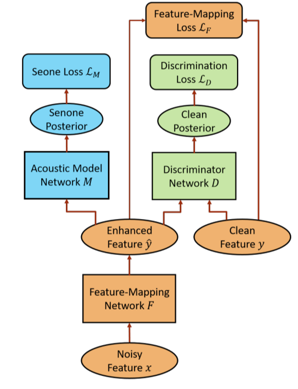
F (G) 的结构与D的结构

F is an LSTM-RNN with 2 hidden layers and 512 units for each hidden layer. A 256-dimensional projection layer is inserted on top of each hidden layer to reduce the number of parameters. F has 87 input units and 29 output units.

The discriminator D is a feedforward DNN with 2 hidden layers and 512 units in each hidden layer. D has 29 input units and one output unit.

The LSTM M has 4 hidden layers with 1024 units in each layer. A 512-dimensional projection layer is inserted on top each hidden layer to reduce the number of parameters. The output layer has 3012 output units predicting senone posteriors.

F的输入输出及D的输入输出

F输入输出Log Mel filterbank (LFB) features

D和M输入LFB，输出概率

损失函数

数据集及数据预处理

CHiME3 dataset

文章的创新点

加了一条Acoustic Model Network的flow用于提升模型对ASR的帮助

MetricGAN: Generative Adversarial Networks based Black-box Metric Scores Optimization for Speech Enhancement

ICML 2019

National Taiwan University

G的结构

BLSTM with two bidirectional LSTM layers, each with 200 nodes, followed by two fully connected layers, each with 300 LeakyReLU nodes and 257 sigmoid nodes for mask estimation, respectively.

G的输入输出

The input features for G is the normalized noisy magnitude spectrogram utterance

D的结构

CNN with four two dimensional (2-D) convolutional layers with the number of filters and kernel size as follows: [15, (5, 5)], [25, (7, 7)], [40, (9, 9)], and [50, (11, 11)]
2-D global average pooling layer was added such that the features can be fixed at 50 dimensions (50 is the number of feature maps in the previous layer)
Three fully connected layers were added subsequently, each with 50 and 10 LeakyReLU nodes, and 1 linear node
D is constrained to be 1-Lipschitz continuous by spectral normalization

D的输入输出

见创新点

损失函数

数据集及数据预处理

TIMIT Dataset

文章的创新点

The main difference between the proposed MetricGAN and the conventional CGAN is how the discriminator is trained. Here, we first introduce a function $Q(I)$ to represent the evaluation metric to be optimized, where $I$ is the input of the metric. For example, for PESQ and STOI, $I$ is the pair of speech that we want to evaluate and the corresponding clean speech $y$. Therefore, to ensure that D behaves similar to Q, we simply modify the objective function of D:

Because we can always map Q to Q’, which is between 0 and 1 (here, 1 represents the best evaluation score), Eq. (3) can be reformulated as:

这篇文章不论是创新点还是实验都很好，值得多读几遍，github也有实现的代码，nice！！！

把D变成evaluator的想法太赞了

项目地址

https://github.com/JasonSWFu/MetricGAN

Speech Enhancement Using Forked Generative Adversarial Networks with Spectral Subtraction

INTERSPEECH 2019

Clemson University (克莱姆森大学)

跳转

文献阅读: Speech Enhancement Using Forked Generative Adversarial Networks with Spectral Subtraction

Sergan: Speech Enhancement Using Relativistic Generative Adversarial Networks With Gradient Penalty

ICASSP 2019

Ghent University, Belgium (比利时根特大学)

G的结构、输入输出与loss

同Segan，但没有随机噪声

D的结构

同G的decoder

D的输入输出

cGAN的输入输出

D的loss

relativistic loss加一个gradient penalty

数据集及数据预处理

voicebank+DEMAND

文章的创新点

文章实验得出了很多有用的结论

这篇文章的实验都是基于segan的，但基本上没有修改segan的G，只是去掉了随机噪声，重要的修改都集中在D上，这里记录几个重要结论

在已有G的基础上简单加D不会有效果，D必须进行精心设计与修改
在D中分别使用VBN和IN，对比说明没有Normalization比较好
不一定BCE就不如LS和Wasserstein loss

项目地址

https://github.com/deepakbaby/se_relativisticgan

UNetGAN: A Robust Speech Enhancement Approach in Time Domain for Extremely Low Signal-to-noise Ratio Condition

INTERSPEECH 2019

Inner Mongolia Key Laboratory of Mongolian Information Processing Technology College of Computer Science, Inner Mongolia Univeristy, Hohhot, China (中国，呼和浩特，内蒙古大学，计算机科学与信息处理技术学院，内蒙古重点实验室)

G的结构

D的结构

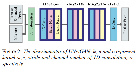
G的输入输出及D的输入输出

waveform及概率

G的loss

D的loss

数据集及数据预处理

TIMIT corpus and NOISEX-92 corpus

文章的创新点

空洞卷积，然后可能实验做得比较好吧

CP-GAN: Context Pyramid Generative Adversarial Network For Speech Enhancementx

ICASSP 2020

Sun Yat-sen University (中山大学)

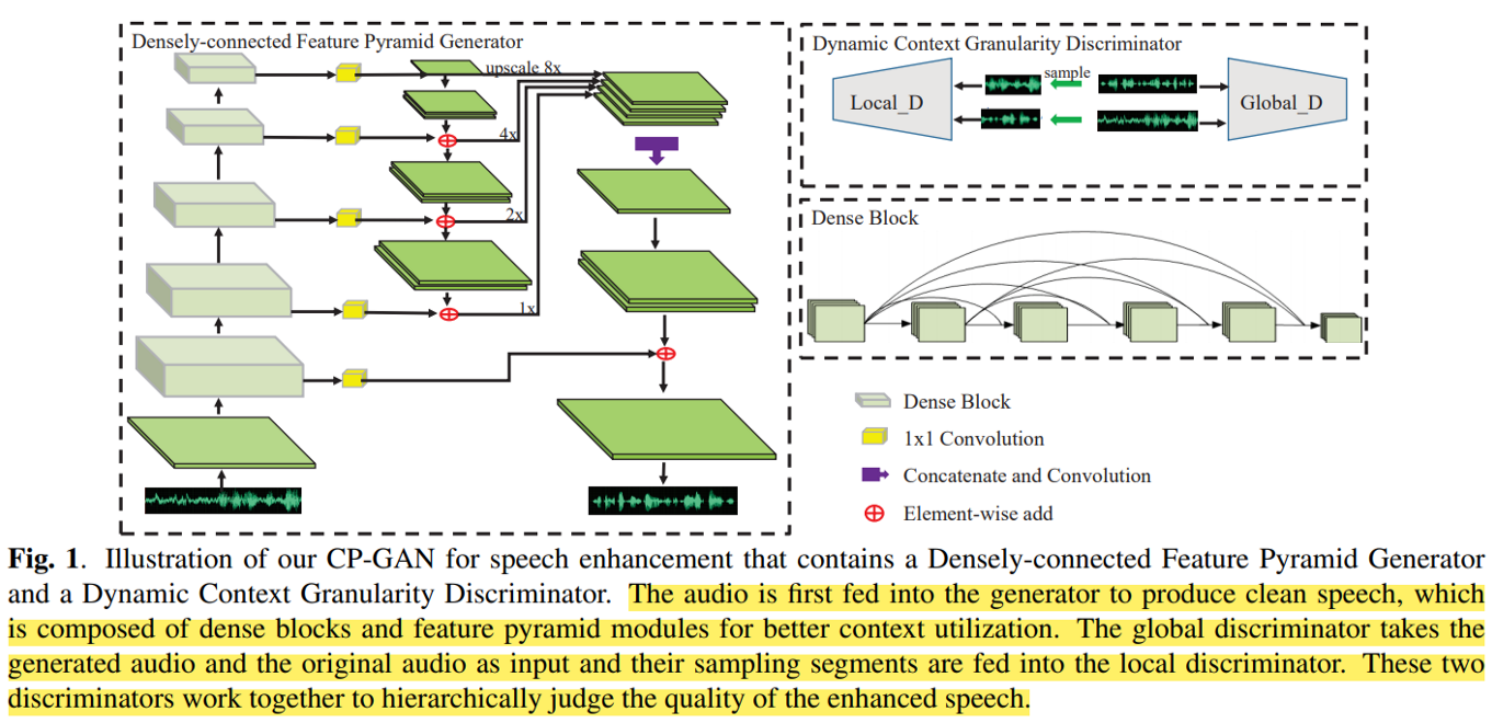
G的结构

FPN backbone use five dense blocks to produce four pyramid features of different scales.
Regarding the generator, five identical dense blocks are cascaded in the bottom-up pathway of FPN and each of the dense blocks contains four convolutional layers. To produce features of different context information, a downsampling (convolution with stride 2) layer is embedded into every dense block. Use skip connection for residual learning before every downsampling operation.
The numbers of output feature maps of these dense blocks are 32, 64, 128, 256 and 512 respectively. In the top-down pathway, [1,1] convolution is incorporated to make all the features of different scales share with the same channels of 128.
The four pyramid features are upsampled to 1/4 size of the original noisy speech signal and then transformed to the features with the channel of 128 by a convolutional layer. Two upsampling layers and one convolutional layer are employed with the output features of the first dense block to generate the enhanced speech signal finally.

G的输入输出

waveform

D的结构

global discriminator: 11 convolutions with stride 2 are employed and a fully connected layer output the probability of a sample being true.
local discriminator: simply five convolutions are utilized, of which the numbers of kernels are 32, 64, 96, 128 and 256. Due to the variable sizes of the input speech signal for local discriminator, we take advantage of the global average pooling following the convolutional layers to produce a fixed-length feature, which is fed into two fully connected layers for classification. The outputs of the final two fully connected layers are 100 and 1. Except for the [1,1] convolution, all of the other convolutional layers have a filter size of 31.

D的输入输出

local_D: 把noisy_wave、gt_wave、enhanced_wave都切割为小segment输入local_D
global_D: 把完整的noisy_wave、gt_wave、enhanced_wave输入global_D

损失函数

损失函数没懂哦

数据集及数据预处理

Voice Bank + DEMAND

Every utterance is segmented by a sliding window of 1 second (16384 samples) with 500 milliseconds (8192 samples) overlapping.